Area source/sink

Area sources or sinks, under Model Build → Area source/sink, are used to distribute extraction/discharge over an area in a domain as opposed to wells and line boundaries, which have extraction/discharge at a point or line. Area source/sink extraction/discharge rates are in units of volume/time/area [L3/T/ L2] = [L/T], like is typical of precipitation or recharge rates. Area source/sinks can represent recharge, vertical leakage, or storage fluxes in transient models. See Recharge, leakage and storage for more discussion.

In steady-state models in domains that are in a single-level part of the model, it can be efficient and appropriate to use a uniform (extraction rate independent of x,y) area source/sink over the entire domain to represent a constant rate of recharge, for example. The Uniform, Domain area source/sink is for such cases. In these cases, the governing equations for aquifer flow are satisfied exactly.

In other cases where the vertical leakage or storage fluxes vary with location (x,y), you'll need to use spatially variable area sinks (SVAS). SVAS are usually needed in multi-level areas of a model, and in transient models.

SVAS and uniform area sinks are mutually exclusive. To avoid this dilemma, no SVAS basis points are placed inside any area that is also covered by a uniform area sink.

Uniform, Domain

With this, the model simulates a constant rate of recharge/leakage over the entire domain.

• Domain defines the domain that the uniform recharge/leakage applies in.
• Top Flux defines the recharge/leakage rate that is applied at the top of the domain, with [L/T] units. This is positive for flux into the aquifer.
• Bottom Flux defines the recharge/leakage rate that is applied at the bottom of the domain, with [L/T] units. This is positive for flux into the aquifer.

Spatially Variable Area Sink Overview

With non-uniform vertical leakage or transient flow, the area source/sink extraction/discharge needs to be spatially variable (varies with x,y) because leakage and/or storage fluxes are not constant over the entire domain. Anaqsim uses multi-quadric interpolator functions to simulate spatially variable area source/sinks (SVAS) (see Fitts (2010) or Strack and Jankovic (1999)). With SVAS, the governing equations of aquifer flow are approximated, and this approximation can be quite good if the density of basis points is high enough (Fitts, 2010). You can check the accuracy of the approximation with Output Specification → Conditions along a Line, which does the same check as shown in Figures 10 and 11 of Fitts (2010).

When you use SVAS, you may assign them over the area of a domain or over the area of a polygon. In either case, SVAS are created in all domains at all levels that are within the area of the specified domain or polygon. If there is a multi-level area of the model, you only input SVAS in one of the levels in the stack. Anaqsim automatically assigns SVAS in the other subdomains that are vertically above or below the ones you specify the SVAS in. When you specify a SVAS by domain or polygon, you specify the condition at the top of the top layer of the model and at the bottom of the bottom layer of the model in the area of the domain or polygon. This condition may be flux-specified, or head-dependent flux -specified. The top or bottom condition may be a specified constant, or it may be defined by an irregular surface.

You have two ways of assigning SVAS and associated basis points:

1. spreading basis points in all model levels at a specified spacing over the area of a domain (Spatially Variable, Domain), and
2. spreading basis points in all model levels at a specified spacing over the area of a polygon (Spatially Variable, Polygon). SVAS polygons are used to refine the top condition, bottom condition, and/or basis point spacing. SVAS polygons first erase any basis points that were inside the polygon and then replaces them at the specified top/bottom conditions and spacing.

In addition, you can refine basis point spacing (but not top/bottom conditions) in the near vicinity of wells (Spatially-Variable, Well Basis Points). This places basis points with an efficient radial, logarithmic spacing to achieve accurate solutions near wells.

The spatially-variable area sink functions are smooth within a domain, but can change abruptly across a domain boundary. An example of this is the pond boundary in the example model in the Fitts (2010) paper. This is a nice feature because at some boundaries like the pond shoreline, you want the extraction to change abruptly.

The rules governing SVAS specifications are summarized below:

• No SVAS are allowed in domains that have uniform area sinks.
• No SVAS basis points are placed in areas also covered by uniform area sinks.
• SVAS-polygon specifications overwrite SVAS-domain specifications, where they overlap.
• SVAS-polygon specifications with a higher nesting level overwrite SVAS-polygon specifications with a lower nesting level.
• The basis point spacings defined with the SVAS-well feature overwrite SVAS-domain and SVAS-polygon basis point spacings, but do not alter the top and bottom conditions in the well vicinity.

Spatially Variable, Domain

This sets up a spatially-variable area source/sink over a whole domain with a uniform spacing of basis points. The governing equation is met perfectly at the basis points, which are distributed on hexagonal centers at the specified spacing. The governing equation is approximated in between basis points.

• Domain defines the domain that the spatially-variable area source/sink applies in.
• Condition Top defines the type of condition that applies at the top of the domain. This is either flux-specified (e.g. a specific recharge rate) or head-dependent flux-specified (e.g. leakage from a lake into the underlying domain). With the latter condition, the source/sink extraction rate is computed using the head difference between a specified head and the domain head, and the vertical resistance to flow offered by the upper or lower half of the domain, in accordance with Darcy’s Law.
• Top Flux or Head defines the flux (flux-specified) or head (head-dependent flux-specified) at the top of the domain. This applies throughout the domain. In transient simulations, this parameter may vary from one time period to the next. If you select "none" under Top Surface, the value specified here applied over the entire area of the domain. If you select a surface instead of "none" under Top Surface, the value specified here is a multiplier that scales the surface (see description below under Top Surface). If you want to use the surface values directly, enter "1.0" here. If, for example, you want to use double the values of the surface as your top flux, enter "2.0" here.
• Top Surface allows you to define a surface for a spatially-variable top condition. This could be used to represent an irregular distribution of recharge at the top of the model, or an irregular distribution of head in an aquifer below the model which the lowest model level leaks to/from. To use this feature, you must first define the surface under Area source/sink → Surfaces for top/bottom conditions. Once you have created the surface, you may select it in the drop-down list that appears in this column. Your choices will be "none" (just use the specified constant value under Top Flux or Head), or one of the previously-defined surfaces. If you choose a surface, the value of the top/bottom condition flux (flux-specified) or head (head-dependent flux-specified) will be equal to the value of the surface at x,y times the number entered under Top Flux or Head. If you select a surface and put "1.0" in the Top Flux or Head field, the value at x,y, will be the value at x,y in the specified surface. If you had entered "1.3" in the Top Flux or Head field, the value at x,y, will be the value at x,y in the specified surface * 1.3. When you have a surface selected, the Top Flux or Head field becomes a multiplier that allows you to scale the magnitude of the surface used in the model. In transient models, you can vary this scaling factor from one time period to the next by entering multiple values separated by commas (see this guidance for transient inputs)
• Condition Bottom defines the type of condition that applies at the bottom of the domain and is analogous to the Condition Top (see above).
• Bottom Flux or Head defines the flux (flux-specified) or head (head-dependent flux-specified) at the bottom of the domain, analogous to the Top Flux or Head (see above). This applies throughout the domain. In transient simulations, this parameter may vary from one time period to the next.
• Bottom Surface allows you to define a surface for a spatially-variable bottom condition, and is analogous to the Top Surface (see above).
• Node Spacing defines the distance between basis points in the spatially-variable area source/sink. Smaller numbers here improve the approximation of the governing flow equations, at the cost of more computation. The appropriate spacing of nodes depends on the transmissivity of the domains and on the vertical conductances involved with the domain, and on how abruptly heads vary with position. A parameter called the leakage factor [L] can provide useful guidance for assigning basis point spacing. For more discussion of appropriate node spacing and the leakage factor, see Strack and Jankovic (1999) or Hansen (2002). The guidance in these papers recommends basis point spacings on the order of the leakage factor to 2x or 3x the leakage factor. Checking extraction with Output Specification → Conditions along a Line is the best way to know if your spacing is small enough for a satisfactory approximation of the governing equations. The two curves in the extraction plot will not deviate significantly if the basis point spacing is small enough.

Spatially Variable, Polygon

This modifies spatially-variable area source/sinks within a polygonal area. This can be used in addition to the Spatially Variable, Domain option to make the spacing of basis points denser in some areas, and to specify different flux or head-dependent flux conditions in some areas.

• Label is a text label that helps you keep track of multiple spatially variable, polygon area source/sinks.
• Nesting Level is a parameter that allows you to nest several spatially variable, polygon area source/sinks inside each other. If you are not nesting or overlapping these Spatially Variable, Polygon features, specify 1 for this. If you want to place a smaller polygon with denser basis point spacing inside another polygon with less dense spacing, use nesting level 1 for the larger polygon and nesting level 2 for the smaller one inside of it. You may nest up to 5 levels to drill down to finer basis point spacing in the key areas (e.g. near a well). The polygons with the higher nesting level overwrite the basis point spacing and flux condition of polygons with lower nesting levels.
• Condition Top, Top Flux or Head, Top Surface, Condition Bottom, Bottom Flux or Head, Bottom Surface, and Node Spacing are all the same as defined for Spatially Variable, Domain area source/sinks.
• Coordinates defines the coordinates of the closed polygon, inside of which the specified flux and node spacing apply. The polygon is automatically closed from the last vertex listed to the first one listed here. Click the edit icon in this cell to open the coordinate editor, and enter one vertex per line. Reverse Order in the coordinate editor reverses the vertex order. To digitise the polygon on the map, click the draw icon and then click each vertex; double-click to close the polygon.

Spatially Variable, Well Basis Points

Here you can define special, efficient spatially-variable area sink (SVAS) basis point spacings that apply near pumping wells, to improve the accuracy of modeled vertical leakage and storage fluxes. The basis points are drawn with density that is high near the well and decreases with radial distance from the well. The closest basis points to the well are placed at a radius two times the radius of the well. Basis points are placed on larger and larger circles out from the well, where the distance between circles increases logarithmically between adjacent circles (like a steady well flow flow-net). The outer limit of these basis points is determined by the Max Node Spacing parameter - circles of basis points continue to be added in the outward direction, until the basis point spacing would exceed Max Node Spacing. Every other circle has all the basis point locations rotated by an angle that is half the angle between basis points on a circle. For example, if you chose 4 Points per Circle, the angle between basis points on a circle would be 360/4 = 90 degrees, and every other circle would have these positions rotated by 45 degrees compared to adjacent circles of basis points (see figures below). These special well basis points replace basis points in this area that were established with SVAS domain or polygon input. The well basis point input only refines the basis point spacing and does not alter the top and bottom conditions that are determined by the SVAS domain or polygon input.

These data are input:

• Well Labels allows you to select which wells this row of input data applies to. You may select one or multiple wells. Make sure all wells in your model have unique labels, so you can identify them in this list.
• Max Node Spacing defines the maximum node spacing at the outer edge of these special basis points. Generally you should have this spacing slightly smaller (about 10-30% less) than the background basis point spacing for the well vicinity.
• Points per Circle defines how many basis points will be placed on each circle around the well. Chose from the drop-down list. A higher number here will make the approximation of storage fluxes and vertical leakage near the well more accurate, but at the expense of more basis points, more equations, and more computation.

The algorithm for placing basis points is illustrated below with a well flow-net plot and basis point placement shown with green triangles for the case of 6 points per circle (basis points shown for 5 outermost circles).

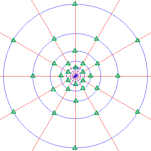
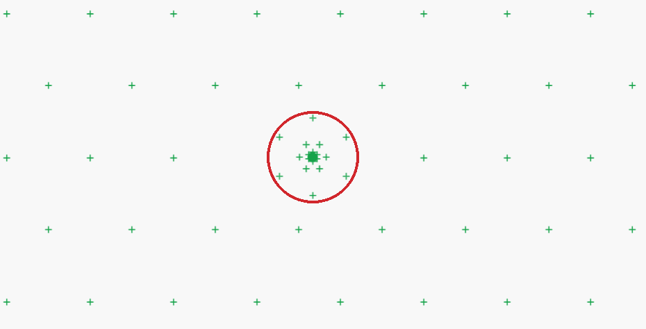
The red circle highlights the denser well basis points around the well. Outside the circle, the regular hexagonal spacing comes from the SVAS domain or polygon inputs.

SVAS Top/Bottom Condition Surfaces

This allows you to input a surface, so that spatially-variable area sink (SVAS) top and bottom conditions can be a assigned using an interpolation function of (x,y) position instead of being constant and independent of (x,y). Some possible applications of this include:

• recharge rate that varies spatially - e.g. more in uplands, less in lowlands.
• irregular distribution of head in an aquifer below the model, which the lowest model level leaks to/from.
• an irregular, sloping freshwater head surface that an interface aquifer leaks toward at the sea shore. The freshwater head increases with depth below sea level, so the specified head condition at the top of an interface domain should be a surface.

The data points that define these surfaces do not correspond to basis points in the SVAS - these data points only define the surface that defines flux or head-dependent flux that is assigned at each basis point. Such surfaces may be referenced by both SVAS, domain and SVAS, polygon input. The surface is created using interpolation between data points that are specified as x,y,value triplets. You must specify at least 3 data points.

If you specify exactly 3 data points, the surface will be a planar surface that passes through each of the 3 points, using the function:

Value(x,y) = Ax + By + C (A, B, C are scalar constants)

If you specify 4 or more data points, the surface is defined using an interpolation function described by Hardy (1971):

Value(x,y) = a1 r1 + a2 r2 + a3 r3 + ... + D (a1, a2 ,a3... and D are scalar constants and r1, r2 ,r3... are radial distances from each (x,y) data point)

This surface passes through each data point and is a smooth but irregular surface.

• Label is a text label that helps you keep track of multiple SVAS top/bottom condition surfaces.
• Surface Data Points defines the list of x,y,value triplets that define the surface. Open the surface data editor and enter the points in a comma-delimited, tab-delimited, or space-delimited form like the following:
  x1, y1, value1
  x2, y2, value2
  x3, y3, value3
  x4, y4, value4
  ...

You can type the points, or paste a block of cells from a spreadsheet into the editor.

When you use a surface for an SVAS top or bottom condition, be sure to read about how the surface is scaled by the number(s) you input for the Top Flux or Head in the SVAS domain or SVAS polygon input.