Display settings

Select Display settings in the toolbar above the map. Use Layer visibility to choose what is shown and the other tabs to configure background maps, reference layers, and solved results.

Layer visibility

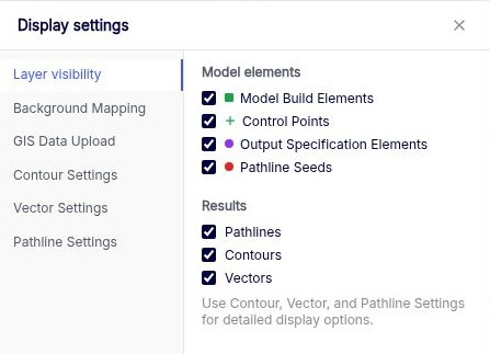
Checkbox	What it shows
Model Build Elements	The elements that define the model, such as domains, boundaries, and wells.
Control Points	Anaqsim displays two types of control points. Line boundaries. The solver enforces the boundary conditions exactly at these points along each line segment. Parameters per Line in the relevant line boundary data table sets the number of points per segment. Spatially variable area sources and sinks. The Spacing column in the corresponding area source or sink data table sets the distance between control points.
Output Specification Elements	Features such as hydrograph points, conditions along a line, and calibration targets.
Pathline Seeds	The starting locations for pathlines.
Pathlines	Toggles visibility for all pathlines on the map. Use Show in the pathline input table to control which individual pathline sets appear.
Contours, Vectors	Toggle the corresponding results from the solve independently.

Background Mapping

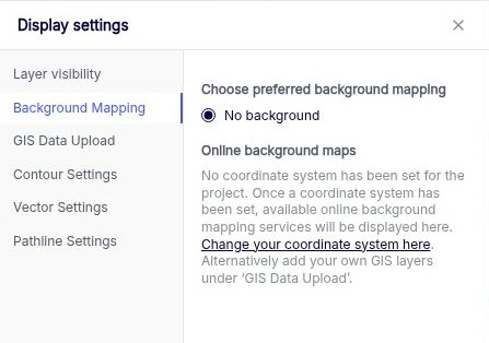
Choose an online background map from the services available for the project’s coordinate system. Choose No background to view the model without an online base map.

If the project has no coordinate system, select Change your coordinate system here to open the project setting. You can also add your own reference data under GIS Data Upload.

GIS Data Upload

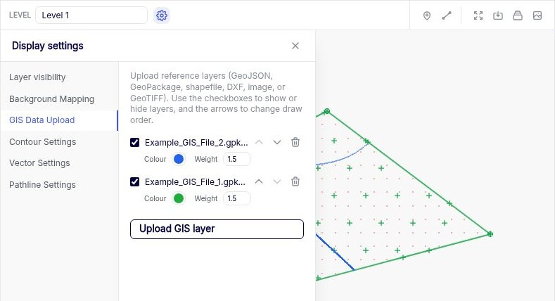
Select Upload GIS layer to add reference data. Supported data types are GeoJSON, GeoPackage, shapefile, DXF, image, and GeoTIFF.

Use a layer’s checkbox to show or hide it and the up and down arrows to change the draw order. Raster layers can also have a greyscale control. These layers provide context for the model on the map.

Place an Image

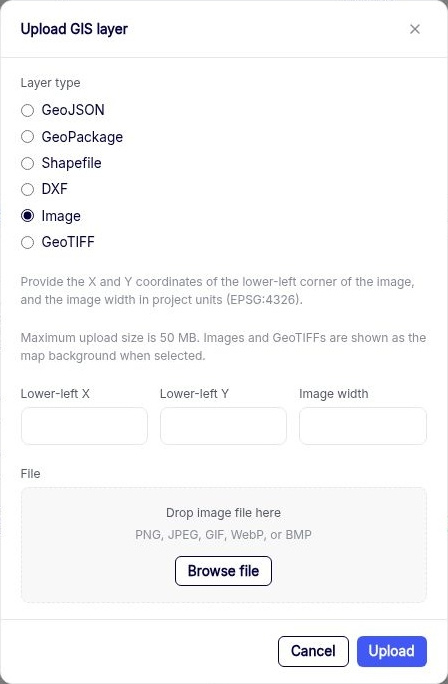
1. Select Image as the layer type. Supported formats are PNG, JPEG, GIF, WebP, and BMP.
2. Enter Lower-left X, Lower-left Y, and Image width in the project’s coordinate units. These define the image’s lower-left corner and width on the map.
3. Use Browse file or drop the image into the form, then select Upload. The maximum upload size is 50 MB.
4. Select the uploaded image to use it as a map background.

Contour Settings

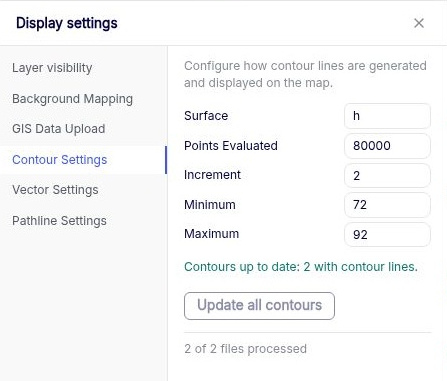
Choose Surface to set what is contoured.

Option	What is contoured
h	Hydraulic head in the selected level.
dh	Head in the selected level minus head in the level below. For example, at Level 1 this compares Levels 1 and 2. Use it to look for vertical head gradients.
extraction	Areally distributed discharge per unit area due to leakage and storage fluxes.
interface	Interface elevation in a fresh/salt interface model.

Setting	What it controls
Points Evaluated	The number of points at which Anaqsim evaluates the surface before contouring. More points can give smoother, more detailed contours and take longer to process.
Increment	The difference between adjacent contour levels, in the units of the selected surface. Use 0 for automatic spacing.
Minimum and Maximum	The lowest and highest contour levels to draw. Leave either blank to let Anaqsim set that end of the range from the surface values.

For example, with a minimum of 72, a maximum of 92, and an increment of 2, Anaqsim draws levels at 72, 74, 76, and so on up to 92 where the surface reaches those values.

After editing the settings for a solved model, select Update all contours when enabled. Check Contours under Layer visibility to show them on the map.

Vector Settings

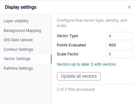
Anaqsim computes flow vectors at points across the plotted area and centres each vector on its evaluation point.

Setting	What it controls
Vector Type	v is average linear velocity, q is specific discharge, and Q is domain discharge. v and q have units of length per time. Q equals q times the saturated thickness and has units of area per time.
Points Evaluated	The number of points where vectors are calculated and displayed. Use fewer points if the plot is crowded.
Scale Factor	The length of the plotted vectors. Larger factors draw longer vectors. At 1, the largest vector is scaled to the spacing between evaluation points.

Select Update all vectors when enabled to regenerate the vectors from the solution. Check Vectors under Layer visibility to display them.

Pathline Settings

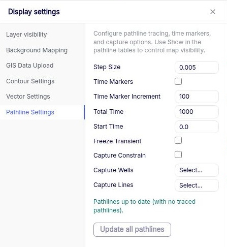
These settings apply to all pathlines. Define the starting points and tracing direction under Output Specification → Pathlines. See Pathline inputs for the available starting geometries.

Tracing and time markers

Setting	What it controls
Step Size	The length of each straight tracing segment as a fraction of the larger horizontal dimension used for tracing. A smaller fraction gives a smoother, more accurate trace and increases computation time.
Time Markers	Draws arrows at regular intervals of elapsed travel time along each pathline.
Time Marker Increment	The time between arrows, in the model’s time units. Applies when Time Markers is on.
Total Time	The maximum travel time to trace. Use it, for example, to plot the extent of a two-year well capture zone.
Start Time	The simulation time at the seed in a transient model. Simulation time decreases along an upstream trace and increases along a downstream trace.
Freeze Transient	Traces through the flow field at Start Time as if it were steady. With this option off, tracing follows the changing flow field through the simulation.

A pathline can end before Total Time if it leaves the model or is captured by a sink. In an unfrozen transient model, tracing also ends at the beginning or end of the simulated time window.

Capture options

Enable Capture Constrain to display only downstream pathlines that are captured by the selected features. Use Capture Wells → Select... or Capture Lines → Select... to choose the wells or internal line boundaries. For example, seed downstream pathlines across a recharge area and select a pumping well to see which starting locations contribute water to it.

Select Update all pathlines when enabled to retrace the pathlines. Use Pathlines in Layer visibility and Show in the pathline tables to control which traces are displayed.