Line boundaries

Line boundaries are under Model Build → Line boundaries. A variety of line boundary conditions are available. Each line boundary is a multi-segmented line (polyline) and the user inputs a list of vertexes in sequence from one end of the polyline to the other. The line boundary condition is approximated using linesink elements similar to those described by Jankovic and Barnes (1999).

Most line boundaries have a parameter that varies from one value at the starting vertex to another value at the ending vertex. The interpolation scheme between the end points is described in the next topic.

Anaqsim approximates the specified boundary conditions along line boundaries, as discussed by Fitts (2010). Check that approximation with the check icon on the line's data row, or by right-clicking the boundary on the map and selecting Check.

For internal line boundaries, the coordinates of all polyline points must not be outside the subdomain boundary, otherwise numerical havoc will be wreaked! It is possible for the start or end point of an internal line boundary to coincide exactly with a corner point of an external line boundary.

Input Common to all Line Boundaries

The following input items are common to all of the line boundaries:

• Label is a text label that helps you keep track of multiple line boundaries.
• Each line segment has a line element with a certain number of unknown parameters that is defined in the Parameters per Line column. If you choose 1 for this, the strength of the element is constant along the line, if you chose 2 for this, the strength of the element varies linearly along the line, if you choose 3 for this, the strength of the element varies parabolically along the line, etc. Using more parameters per line can increase the accuracy of the boundary condition approximation along the line, but at the cost of additional equations in the system of equations that is solved. You only need a high number of parameters per line if the heads or discharges along the element are expected to vary complexly. In many cases, 3 or fewer parameters per line is plenty. Experiment with this and reduce the number of parameters to the minimum that gives you reasonable boundary condition accuracy, which you can check with the check icon on the row. In the case of a Discharge-Specified line boundary, the user does not define Parameters per Line because it is always set to 1; the discharge/length of these line elements is constant and equal to the specified discharge of the line boundary divided by its total length.
• Coordinates defines the x,y coordinates of the polyline vertexes. Click the edit icon in this cell to open the coordinate editor, and enter one vertex per line, with x and y separated by a comma or a tab. You can paste coordinates into that editor. Reverse Order in the coordinate editor reverses the vertex order, which is useful if they were entered in the wrong direction. To digitise the line on the map, click the draw icon and then click each vertex; double-click to finish. The coordinates in the table update. For a normal flux-specified external boundary, list the coordinates counter-clockwise, with the domain to the left as you proceed along the boundary.

Most line boundaries have additional parameters defined at the start and end points, such as heads for head-specified line boundaries. With all such parameters, the same algorithm is employed to interpolate the specified values along the line boundary:

1. Apportion the intermediate values to the vertexes based on the number of line segments in the polyline. For example, if there are 4 segments and the end values are 100 and 110, the values at the vertexes would be 100, 102.5, 105, 107.5, and 110. If there are 5 segments, the values at the vertexes would be 100, 102, 104, 106, 108, and 110.
2. Linearly interpolate values to the control points within a line segment, assuming a linear distribution from one end to the other.

The additional parameters specific to each type of line boundary are listed in the following topics.

Head-Specified

With head-specified line boundaries you specify these additional items:

• Domain defines the domain that the line boundary is in. Choose the domain from the list in this cell.
• Check the Domain Boundary check box if this line boundary is on the external boundary of the domain.
• The h Start and h End are the specified head values at the starting and ending vertexes. In transient simulations, these parameters may vary from one time period to the next.
• Off Periods sets the line boundary discharge to zero during the listed periods of a transient simulation. This can be useful for a dewatering trench that is turned off and on. Separate multiple period numbers with commas. In the example below, the boundary is off in period 2 and uses start and end heads of 94.1 and 93.2 when active.

Boundary condition equations are written at each control point on each line segment. The equation specifies that the modeled head = specified head (interpolated between endpoints of the line boundary). The specified head condition is approximated between control points and may be checked with the check icon on the row.

Normal Flux-Specified

With normal flux-specified line boundaries you specify these additional items:

• Domain defines the domain that the line boundary is in. Choose the domain from the list in this cell.
• Check the Domain Boundary check box if this line boundary is on the external boundary of the domain.

Warning

When the boundary is external, it is necessary to list the coordinates of the polyline in counter-clockwise order with the domain to the left of the boundary as you proceed along it. If coordinates are specified in the wrong (clockwise) order, there is a check in the program that will detect and report this error. This error can occur if you mistakenly specified the coordinates in clockwise order around the outside of the domain. This message can also result if you have made errors in specifying additional external line boundaries either at these same coordinates (e.g. have two external line boundaries in the input that share the same vertex coordinates), or have erroneous external line boundaries to the right of this one (see discussion of left/right algorithm).

• The Normal Flux Start and Normal Flux End are the specified normal flux values at the starting and ending vertexes. Normal flux is the component of domain discharge normal to the line segment, and has units of discharge per length [L³/T/L] = [L²/T]. This may also be thought of as the normal component of specific discharge times saturated thickness. The normal flux is positive for flow across the boundary from left to right as you proceed from the start toward the end. Normal flux is negative for flow from right to left as you proceed from the start toward the end. In transient simulations, the normal flux parameters may vary from one time period to the next.

Boundary condition equations are written for sub-intervals in each line segment (e.g. three subintervals for 3 parameters/line). The equation specifies that the total discharge across the line over the subinterval equals the total to interpolated specified fluxes over the interval. The accuracy of this approximation may be checked with the check icon on the row.

Head-Dependent Normal Flux (3rd type)

This allows head-dependent normal flux into or out of the model, depending on the modeled head at the boundary. Boundary conditions like this are sometimes called 3rd type, Robin, general head (GHB in MODFLOW), or mixed boundary conditions; they involve both head and flux. The boundary must be an external boundary of a domain. It is necessary to list the coordinates of the polyline in counter-clockwise order with the domain to the left of the boundary as you proceed along it. If coordinates are specified in the wrong order, there is a check in the program that will detect and report this error. This error can occur if you mistakenly specified the coordinates in clockwise order around the outside of the domain. This message can also result if you have made errors in specifying additional external line boundaries either at these same coordinates (e.g. have two external line boundaries in the input that share the same vertex coordinates), or have erroneous external line boundaries to the right of this one (see discussion of left/right algorithm).

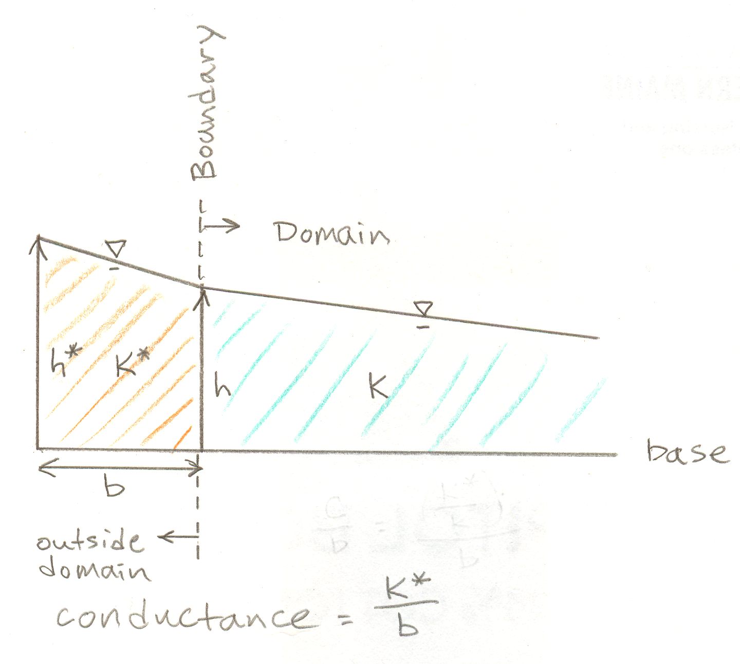
This kind of boundary is illustrated conceptually in the vertical profile sketched below. It is as though there is a fictional domain beyond the boundary (orange) outside of the domain (blue) , and at a distance b outside the boundary, there is a fixed head h*. The head difference between h* and the head at the boundary (h) drives a component of discharge normal to the boundary.

You specify these additional items with this type of boundary:

• Domain defines the domain that the line boundary borders. Choose the domain from the list in this cell.
• Conductance Start and Conductance End = K*/b at the starting and ending vertexes, where b is the horizontal width of the fictional domain normal to the line boundary and K* is the fictional domain horizontal K*. When K*/b is smaller, there is low conductance at this boundary and the normal component of discharge is smaller. The entry for Conductance End can be "=start" if you want the same conductance for the entire line boundary. Alternatively, the entry for Conductance End can be "=start*D" if you want the Conductance End to be equal to Conductance Start times the real constant D. Using "=start" or "=start*D" is particularly handy for parameter estimation, to limit the number of parameters being estimated. Prior to release 2016-3, the conductance parameter for this kind of line boundary was defined as C/b = (K*/b/K), which differs from this conductance by the factor K, which is the K of the domain. When a domain is anisotropic in the plane of the domain, the factor K = (K1 * K2)1/2.
• h* Start and h* End are the specified head values at the starting and ending vertexes, representing head a distance b outside the boundary.

The component of aquifer discharge normal to the boundary is Q_n [L²/T], determined by this equation:

\[ Q_n = (K^*/b/K)(\Phi - \Phi^*) \]

Where Φ* is the aquifer discharge potential computed for the domain using h*, and Φ is the aquifer discharge potential computed using modeled h at the boundary. Q_n is positive for discharge out of the domain. The equation relating h to Φ depends on the domain type - it is a linear relation for confined domains but is nonlinear for unconfined and interface domains. Books describing Φ(h) equations in the analytic element method include Fitts (2023), Strack (1989), and Haitjema (1995). By writing the boundary condition equation this way, the boundary condition is linear, even when Φ(h) is nonlinear.

For a confined isotropic domain, the normal component of aquifer discharge is:

\[ Q_n = (K^*/b/K) * T * (h - h^*) \]

Where T is the transmissivity of the domain and h is the modeled head at the boundary.

For an unconfined isotropic domain, the normal component of aquifer discharge is:

\[ Q_n = (K^*/b/K)\left(\frac{K}{2}\right)\left(h^2 - h^{*2}\right) \]

Where K is the horizontal K of the domain, and h and h* are measured from the base of the domain.

The boundary condition equation

\[ Q_n = (K^*/b/K)(\Phi - \Phi^*) \]

is written at each control point on each line segment. The values of conductance and Φ* are interpolated between the values specified at the start and end of the boundary. The modeled boundary condition is approximated between control points and may be checked with the check icon on the row.

Discharge-Specified

With discharge-specified line boundaries you specify these additional items:

• Domain defines the domain that the line boundary is in. Choose the domain from the list in this cell.
• Discharge of the entire polyline in volume/time units [L³/T].

With this type of line boundary, the discharge per length of line is constant along the entire length of the polyline. Negative discharge implies extraction from the aquifer and positive discharge implies injection into the aquifer. In transient simulations, this parameter may vary from one time period to the next. This type of line boundary must always be internal, not on the external boundary of a domain. To specify discharge into or out of the external boundary of a domain, use Normal Flux-Specified boundaries.

River

With river line boundaries you specify these additional items:

• Domain defines the domain that the line boundary is in. Choose the domain from the list in this cell.
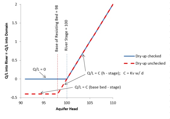
• Check the Dries Up check box if this river boundary is allowed to dry up (revert to zero discharge per length) when the head falls below the specified stage. Check Dries Up in cases where the river is small and would dry up if aquifer heads drop below stage. If Dries Up is not checked, the river’s discharge is computed based on a head difference and a river bed conductance factor in accordance with Darcy’s Law. There are two possibilities for how the head difference is computed: 1) if the domain head is above the base of the resisting bed, then it is the difference between the stage and the head in the domain, and 2) if the domain head is below the base of the resisting bed, then it is the difference between the stage and the elevation of the base of the resisting bed. The following graph illustrates how the discharge/length to the river line boundary would vary with or without Dries Up checked, for the following assumptions: stage = 100, resisting bed base = 98, resisting bed conductance C = K_v w / d = 0.2.

• Stage Start and Stage End are the specified river stages (water surface elevations) at the starting and ending vertexes. In transient simulations, these parameters may vary from one time period to the next.
• Conductance Start and Conductance End are the specified river bed conductance factors at the starting and ending vertexes. The conductance factor equals K_v w/d where K_v is the vertical hydraulic conductivity of the resistant river bed, w is the horizontal width of the river bed, and d is the thickness of the resistant river bed. Kv w/d has units of [L/T]. The entry for Conductance End can be "=start" if you want the same conductance for the entire line boundary. Alternatively the entry for Conductance End can be "=start*D" if you want Conductance End to be equal to Conductance Start times the real constant D. Using "=start" or "=start*D" is particularly handy for parameter estimation, to limit the number of parameters being estimated.
• Base Resisting Layer Start and Base Resisting Layer End are the specified elevations of the bottom of the river bed resisting layer at the starting and ending vertexes.

Boundary condition equations are written at each control point on each line segment. The equation specifies that the discharge/length of the linesink be related to the stage and conductance(interpolated between endpoints of the line boundary) as described above. The specified head condition is approximated between control points and may be checked with the check icon on the row. In the graphical check, the sign of the discharge is negative for flow from the domain to the river, consistent with other discharging elements.

Drain/Fracture

Drain/Fracture line boundaries allow modeling of thin features like drains or fractures that conduct water at a high rate compared to the surrounding domain. The drain or fracture is represented in the model as a line with zero actual width using line dipole functions. With these line boundaries, specify these additional items:

• Domain defines the domain that the line boundary is in. Choose the domain from the list in this cell.
• Conductance Start and Conductance End = bK* at the starting and ending vertexes, where b is the horizontal width of the drain normal to the direction of the line, and K* is the drain hydraulic conductivity. This formulation assumes the drain fully penetrates the domain. The entry for Conductance End can be "=start" if you want the same conductance for the entire line boundary. Alternatively the entry for Conductance End can be "=start*D" if you want the Conductance End to be equal to Conductance Start times the real constant D. Using "=start" or "=start*D" is particularly handy for parameter estimation, to limit the number of parameters being estimated. Prior to release 2016-3, the conductance parameter for this kind of line boundary was defined as bR = (bK*/K), which differs from this conductance by the factor K, which is the K of the domain. When a domain is anisotropic in the plane of the domain, the factor K = (K1 * K2)^1/2.

Boundary condition equations are written at each control point on each line segment. The equation specifies that the modeled discharge within the drain (jump in stream function across drain) equals Conductance/K (interpolated between endpoints of the line boundary) times the gradient of the aquifer discharge potential in the direction of the drain. This condition is approximated between control points and may be checked with the check icon on the row. In the graphical check, the discharge is positive for flow from the start of the boundary toward the end of the boundary, as defined by the order of vertexes. To achieve better accuracy of this approximation, use shorter line segments and/or more parameters/line. Shorter segments are particularly helpful at the ends of the line boundary, where the boundary condition changes rapidly.

Leaky Barrier

Leaky Barrier line boundaries allow modeling of thin features like sheet pile walls or slurry walls that create a barrier to flow, but allow some leakage. The leaky barrier is represented in the model as a line with zero actual width using line doublet functions. With these line boundaries, specify these additional items:

• Domain defines the domain that the line boundary is in. Choose the domain from the list in this cell.
• Conductance Start and Conductance End = K*/b at the starting and ending vertexes, where b is the width of the barrier normal to the direction of the line, and K* is the horizontal conductivity of the barrier. It is assumed that the barrier fully penetrates the domain. The entry for Conductance End can be "=start" if you want the same conductance for the entire line boundary. Alternatively the entry for Conductance End can be "=start*D" if you want the Conductance End to be equal to Conductance Start times the real constant D. Using "=start" or "=start*D" is particularly handy for parameter estimation, to limit the number of parameters being estimated. Prior to release 2016-3, the conductance parameter for this kind of line boundary was defined as R/b = (K*/b/K), which differs from this conductance by the factor K, which is the K of the domain. When a domain is anisotropic in the plane of the domain, the factor K = (K1 * K2)^1/2.

Boundary condition equations are written at each control point on each line segment. The equation specifies that the modeled aquifer discharge component normal to the barrier equals Conductance/K (interpolated between endpoints of the line boundary) times the jump in aquifer discharge potential across the barrier. This condition is approximated between control points and may be checked with the check icon on the row. In this check, discharge is positive for flow going from left to right as you proceed along the boundary from the start towards the end. To achieve better accuracy of this approximation, use shorter line segments and/or more parameters/line. Shorter segments are particularly helpful at the ends of the line boundary, where the boundary condition changes rapidly.

Inter-Domain

Inter-domain line boundaries define the boundaries between abutting domains. It is possible to use these boundaries to abruptly shift the layering (levels) in the model. For example, there could be a single level on one side of the boundary and multiple levels on the other side. For inter-domain boundaries, you specify these additional items:

• Domains Left defines the domains that are to the left of the boundary as you proceed from the first towards the last vertex listed under Coordinates. Imagine you were on the ground walking along the boundary heading towards the last vertex - the left domains would be on your left and the right domains would be on your right. Choose these domains in the cell.
• Domains Right defines the domains that lie to the right of the boundary as you proceed from the first towards the last vertex listed under Coordinates. Choose these domains in the cell.

It is easy to make a mistake specifying Domains Left or Domains Right, so Anaqsim checks this and will alert you with an error message if it detects an error. This error can occur if you mistakenly specified the left domain(s) on the right or vice versa. This message can also result if you have made errors in specifying additional external line boundaries either at these same coordinates (e.g. have two external line boundaries in the input that share the same vertex coordinates), or have erroneous external line boundaries to the right of this one (see discussion of left/right algorithm).

On one side of the inter-domain boundary, there should be a single domain. The reasons for this are explained in the Anaqsim Modeling Concepts section. At inter-domain boundaries, the domain discharges normal to the boundary are matched so that over sub-segments of each line segment, the total normal discharge of domains to the left matches the total normal discharge of domains to the right. The number of sub-segments per line segment equals the number of parameters per line. The heads in all domains match at control points along the line segment. The number of such control points equals the number of parameters per line. Fitts (2010) provides more discussion of how boundary conditions are approximated at inter-domain boundaries. The accuracy of the modeled boundary conditions may be checked with the check icon on the row.

Head-Specified External with Gradient

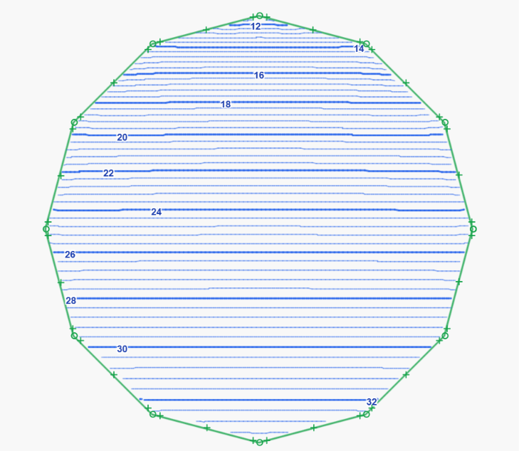
This is a useful line boundary for simple models where you want to impose a uniform groundwater flow across your area of interest, but do not want to specify a lot of other details. Head-specified line boundaries are placed around a roughly circular outer boundary, and the specified heads create a uniform cross-flow in the absence of other elements. This feature creates a 12-sided approximately circular boundary consisting of specified head line boundaries, which forms the entire external boundary of the domain.

With this type of line boundary you specify these additional items:

• Domain defines the domain that the line boundary is external to. Choose the domain from the list in this cell.
• X,Y of origin defines the coordinates of the center of the circle (put at the center of the area of interest).
• Radius is the radius of the circle.
• Gradient is the desired horizontal hydraulic gradient at the center of the circle, in the absence of any other elements.
• Gradient Direction is the angle that the down-gradient direction of the gradient makes with the positive x axis, in degrees.

Boundary condition equations specifying head are written at each control point on each line segment. The specified head condition is approximated between control points and may be checked with the check icon on the row.

In all types of domains, this boundary by itself produces a uniform flow across the circle, with a uniform aquifer discharge (specific discharge * saturated thickness), and head at the center of the circle will equal the Average Head specified for the domain. With a confined domain, the specified gradient will be the gradient everywhere along the circle boundary and everywhere within the circle in the absence of other elements. With unconfined or interface domains and no other elements, the gradient changes with saturated thickness (higher gradient with less saturated thickness), and the specified head gradient will occur at the center and along the midline of the circle.

The contours below show the head distribution produced by this boundary. In an unconfined domain with no other elements, the hydraulic gradient is steeper where the saturated thickness is smaller. The product of saturated thickness and hydraulic gradient stays constant across the domain.